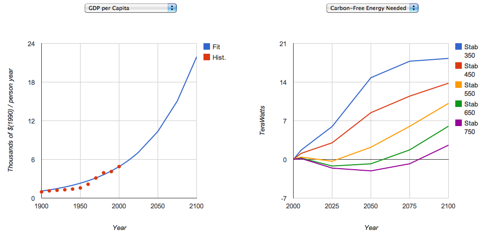
On the left, the GDP per capita as tuned to follow the past historical trend. On the right, amounts of carbon-free energy needed, in teraWatts or 1012 Watts, in order to stabilize atmospheric CO2 at various levels between 750 and 350 ppm.
The other parameters are unchanging with time as the model page loads. Look at the model forecast for each, compared with data, by selecting GDP per Capita for example in one of the two menus just above the plots, or by mousing over the input box underneath the $GDP/person term in the formula. One idea for predicting the future is extrapolating from the past, which means adjusting the growth/decay rate until the solid blue curve is a nice eyeball fit to the red data points. Do the same for the other factors, Watts/$ and CO2/Watt.
This page runs its emissions predictions through the ISAM model to calculate atmospheric CO2 concentration, temperature, and sea level. This page also calculates how much Carbon-free energy would be needed in order to stabilize atmospheric CO2 concentrations at a range of values (750 which is easy, 650, 550, 450, and 350 ppm).
| Find the best-fit values for the various model parameters. This is basically a business-as-usual type of scenario |
| Given the uncertainties in the best-fit parameters (by eyeball fit), what are the best and worst case scenarios for business-as-usual? |
| Construct stabilization scenarios, limiting atmospheric CO2 to, say, 450 ppm. How much carbon-free energy would this require by the year 2100? |
 |
The University of Chicago 5801 South Ellis Ave Chicago IL 60637 773.702.1234 |