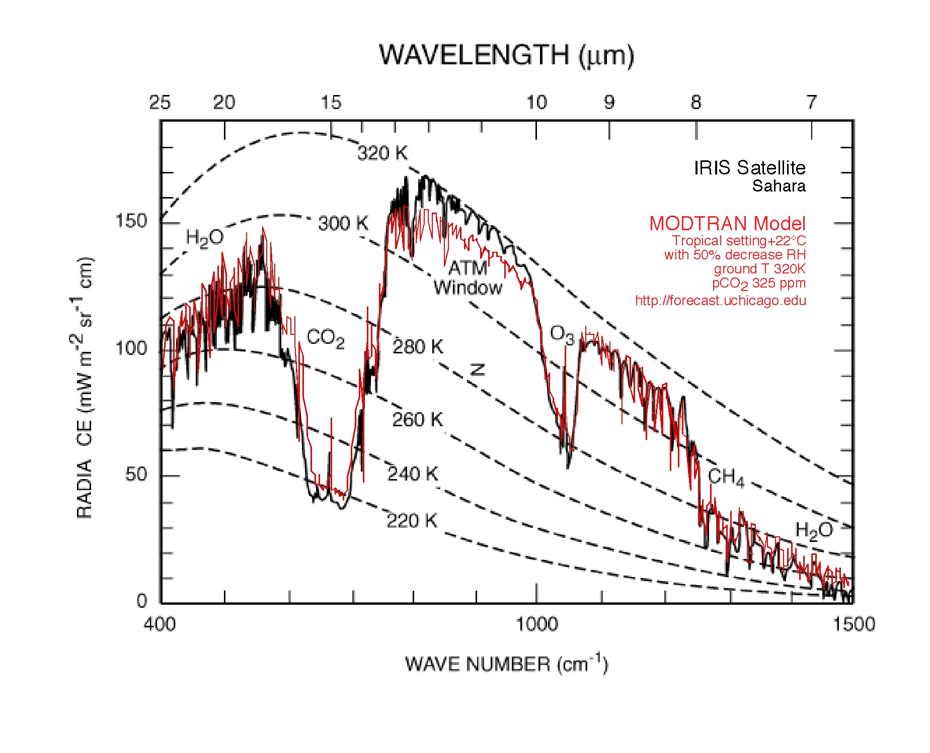
MODTRAN results (red) compared with data (solid black) from the Nimbus 3 IRIS instrumentfrom Hanel et al., 1972).
You can modify the greenhouse gases and weather, and see how it effects the outgoing infrared energy spectrum. The total infrared energy flux leaving the planet is labeled Upward IR Heat Flux. The model does not compute global warming, that is, it doesn't change the Earth temperature in response to changes in the atmosphere. However, you can alter the temperature of the ground and atmosphere yourself to compensate for a change in IR energy flux
The greenhouse gases CO2, methane, and tropospheric ozone can be set by entering concentrations as labeled. Stratospheric ozone and water vapor are scaled by the number in the box (where a value of 1 would take the default value with no change).
Ground Temperature Offset changes the temperature of the ground and the overlying atmosphere by the amount you specify. The change imposed in the atmosphere is not very realistic but gives the first-order behavior, by simply decreasing as much as the ground temperature up to an altitude of 10 km. You can see a atmospheric profiles of temperature, water vapor, and ozone by selecting the options underneath the profile plot.
If you alter the atmospheric temperature you raise the question of what to do with the water vapor. The options appear when T offset is not equal to 0 of Holding Fixed Vapor Pressure (absolute number of vapor molecules) or Holding Fixed Relative Humidity (scaling the vapor pressure by the change in equilibrium vapor pressure as you changed the temperature).
There are several standard atmospheric settings, and standard cloud settings. The Altitude (km) refers to the virtual sensor; if you set this to zero you will see the ground with no atmospheric interference, and if you set it Looking Up you will see the sky by IR.
You can compare two model runs by running the first, then selecting Save This Run to Background. The run will be saved on the plot, and you can superimpose a second by changing model options. Get rid of the backround plot by Deleting it. The default way to plot the spectra are by wavenumber, but you can also view it by wavelength on either linear or log axis. The intensity plotted on the y-axis is an energy flow integrated between two values on the x axis. The different ways of tabulating the light frequencies are nonlinear, so it's as if the plot were being squished around horizontally, squeezing together in some regions and stretching apart in others as you change the plot type. The intensity, representing the area in that integral, gets higher where the plot is geting squeezed, and lower where it is stretched.
| Demonstrate the Band Saturation Effect by making a plot of Iout as a function of a greenhouse gas concentration, from say 0 to 1000 ppm, with lots of points at low concentrations. |
| Calculate the average temperature that the Earth radiates to space by setting the model Iout to epsilon sigma T4 and solving for T. What altitude is this (assuming the light is coming from the troposphere, the lowermost region in the temperature profile plot)? How does this altitude change as you change the greenhouse gas concentration? |
| What is the effect of clouds on the upwelling IR to space, and to the downwelling IR seen from the ground? |
| Compare CO2 vs. methane as greenhouse gases. Which would be the stronger if they had the same concentrations? Which is stronger given their current concentrations? |
| Simulate the temperature response to greenhouse gas IR forcing by adjusting the ground temperature to maintain a constant Iout as you increase the gas concentration. Demonstrate the water vapor feedback effect by doing this using both options of constant vapor pressure and constant relative humidity. |
| Find the model's climate sensitivity. |
 |
The University of Chicago 5801 South Ellis Ave Chicago IL 60637 773.702.1234 |